Journal of Animal Research: v.10 n.1, p. 77-84. February 2020
DOI: 10.30954/2277-940X.01.2020.10
Time Series Investigation of Milk Production in Major States of India Using ARIMA Modeling
ABSTRACT
In India, white revolution was started during 1970's with Operation flood programme. After this revolution, production of milk in India had tremendously increased. Contribution of diary sector has continuously increased in Indian Gross Domestic Product (GDP). Livestock sector has emerged as an essential growth driver of the Indian wealth. This study is associated with time series data of five major milk producing states in 2017-18 in India. The milk production projection has been made using Auto Regressive Integrated Moving average model (ARIMA) for year 2024-25. From the forecasted figures, Uttar Pradesh would be leading states of India in milk production with 37.68 MMT in year 2024-25. Whole India milk production would reach 252.948 MMT in year 2024-25. This projection helps in formulating national agricultural policy as well as proper planning for products into dairy sector.
Keywords: ARIMA, ADF, Forecasting, Milk Production, Time Series
Dairy sector in India is one of the vibrant sectors of India; it has witnessed record growth of 6.7 percent during 2017¬18 (Anonymous, 2018). This phenomenal growth record is also accompanied by its being recognized by NITI AYOG as the prime sector which can help double income of the farmers' in the country. The dairy sector has made excellent performance in exporting high value products to the tune of US $575 million compared to its imports of US $34.6 million and helped India re-emerge as the net exporter of dairy products. In 1970-71, per capita milk availability was 110 gram per day per person which rose to 378 gram per day per person in 2017-18 (Anonymous, 2018). This has significantly contributed to the betterment of food sufficiency of the nation. Despite such impressive performance, milk is luxury for many in India. The milk prices in India are comparatively higher than price prevailing in International market Bhardwaj et al. (2017). Dairies are coming up in traditional milk powerhouses like Haryana, Punjab and Andhra Pradesh. This is a rapidly growing sector and progressively a number of established businesses are examining the feasibility of entering the dairy industry through large commercial farms. The brief and rosy picture depicted by the facts and figures presented above is merely a snapshot of dairy sector performance in India. However, it needs further examination to uncover the finer details of its performance. When policy matters are discussed the nit is important to have estimates of future production that is likely to take place in the country. In this direction, Sharma et al. (2018) investigated the monthly arrival of Rohu fish using ARIMA in Jammu Region of J&K State. Deshmukh and Paramasivam (2016) evaluated about milk production forecasting using ARIMA and VAR time series model. Chaudhari and Tingre (2014) considered about egg production in India using ARIMA modelling. Prajneshu and Venugopalan (1997) identified models to forecast the future fish production. Mishra et al.(2020) used ARIMA modeling in India and Chhattisgarh. At present, India is self-sufficient in milk production. But increasing population also increase the demand for milk and milk made product. The policy making regarding milk production got shot in arm owing to initiatives of Dr. Verghees Kurian, the father of White Revolution in India. The policy makers needs forecast for effective policy decision on variables such as price support to farmers, import and anti-dumping duty and quality improvement programmes. Keeping in mind following objectives are framed for the study: It is necessary to find out what will be the future milk production, so appropriate policy implications can be planned.
How to cite this article: Mishra, P., Fatih, C., Vani, G.K., Tiwari, S., Ramesh, D. and Dubey, A. (2020). Forecasting of milk production in major states of India using ARIMA modeling. J. Anim. Res., 10 (1): 77-84.
MATERIALS AND METHODS
Auto-Regressive Integrated Moving (ARIMA) Approach
Time series is a branch of Statistics; the object is to study variables over time. Among its main objectives is the determination of trends within these series as well as the stability of values (and their variation) over time. Unlike traditional econometrics, the purpose of time series analysis is not to relate variables to one another, but to focus on the “dynamics” of a variable. In particular, linear models (mainly AR and MA, for Auto-Regressive and Moving Average), (Box-Jenkins, 1976), conditional heteroscedasticity models, notably ARCH (Auto¬Regressive Conditional Heteroskedasticity), (Engel, 1982 ) are used in modeling time series . In this study, we deal with Auto-Regressive Integrated Moving (ARIMA) process, (called Box-Jenkins Approach) to estimate and forecast the milk production in India and five major milk producing states namely, Andhra Pradesh, Madhya Pradesh, Uttar Pradesh, Gujarat and Rajasthan, over the period 2001 to 2018. The selection of states was done on the basis of their contribution to milk production in the country in year 2017-18.
These five states contributed nearly 53 percent of total milk production in India. The data for analysis was collected from the Department of Animal Husbandry, Dairying & Fisheries, Ministry of Agriculture and Farmers Welfare, Government of India.
In practice, it is impossible to know the probability distribution of a time series yt,, t > 0; therefore, when primary interested is in the modeling of the conditional distribution (a priori constant in time) of yt,, via its density:
Conditioned on the history of the process: yt = y, y t1,, … y0. It is therefore a necessity to model yt on its past values.
Auto-Regressive Model, AR (p)
The conditional approach in Equation (i) provides a decomposition prediction error, according to which:
Where, Eyy)is the component of y, that can give rise to a forecast, when the history of the process, yt--i, yt--2 ., y 0are known. And ef represents unpredictable information. We suppose, ef~ WN (0, a2), is white noise process. The equation (2) represents an autoregressive model (AR) of order p. As an example an autoregressive processes of order i, AR (i) is defined:

The value yt depends only on its predecessor. Its properties are functions of a which is a factor of inertia. Autoregressive processes AR (p) assume that each observation yt can be predicted by the weighted sum of a set of previous observations yt1,, y-2,,. y , plus a random error term. The other type of process of the box-jenkins approach is Moving Average, MA(q).
Moving-Average process MA (q)
The moving average processes assume that each observation yt is a function of the errors in the preceding observations, et-1, et-2, ..., ztp,, plus its own error. A moving average process is given as:
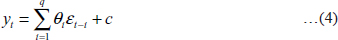
i = 1
The combination of the two models, AR (p) in equation (3) and MA(q) in equation (4) is an ARMA(p, q) process; which is the most popular models of the Box Jenkins for its flexibility and suitability for various data types. The model is designed as follow:
With:
The time series yt must be stationary to be fitted by an ARMA models. We take the case of weak stationary, and we put its definition:
Definition: a time process yt with real values and discrete time y1,, y2,, ... yt.. It is stationary in the weak sense (or “second order”, or “in covariance”) if:
When one or more stationary conditions are not met, the series is said to be non-stationary. This term, however, covers many types of non-stationary, (no-stationary in trend, stochastically non-stationary,...), we focused on the later. Thus, if yt is a stochastically non-stationary, a difference stationary technique should be applied. Consequently, a series is stationary in difference if the series obtained by differentiating the values of the original series is stationary. Generally, we used the KPSS test, (Kwiatkowski et al., 1992 and Leybourne and McCabe, 1994).
The difference operator is given by: A(yt)) = yt-- yt1,, if the series is differentiated d times, we say that it is integrated of order I (d). The process will be noted as ARIMA (p,d,q), defined by the equation:

With, L: is the lag operator (L) or backshift operator (B); If the time series Xt= 1 - L)d yt is stationary, then, estimating an ARIMA (p,d,q), process on yt is equivalent to estimating an ARMA (p, q) process on Xt..
Box and Jenkins (1970) proposed a prediction technique for a univariate series that is based on the notion of the ARIMA process. This technique has three stages: identification, estimation and verification. The first step is to identify the ARIMA model (p, d,q) that could spawn the series. It consists, first of all, in transforming the series in order to make it stationary (the number of differentiations determines the order of integration: d), and then to identify the ARMA model (p, q) of the series transformed with the correlogram and partial correlogram. The graph of autocorrelation (correlogram) and partial autocorrelation coefficients (partial correlogram) give information on the order of the ARMA model. Thus, if we observe that the first two autocorrelation coefficients are significant, we will identify the following model: MA (2). The second step is to estimate the ARIMA model using a non-linear method (nonlinear least squares or maximum likelihood). These methods are applied using the degrees p, d and qfound in the identification step.
Generally, we use the Maximum Likelihood method; by consider that the errors et follow a normal distribution,
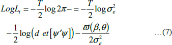
With:
The third step is to check whether the estimated model reproduces the model that generated the data. For this purpose, the residuals obtained from the estimated model are used to check whether they behave like white noise errors using a “portmanteau” test (a global test that makes it possible to test the hypothesis of independence of residues). The common tests are based on residuals analysis for normality, and autocorrelation (Box and Pierce, 1970; Ljung and Box, 1978; Durbin and Watson, 1950 & 1951), Homoskedasticity: Test of Breusch and Pegan (1979), ARCH Test, Engel (1982). The last point under this step is the prediction of future values of yt by the selected model.
RESULTS AND DISCUSSION
We have six time series of milk production: for India at whole, Gujarat, Rajasthan, Andhra Pradesh, Madhya Pradesh and Uttar Pradesh over the period (2001-2018). Table 1, provides summary statistics for milk production data of major states of India. From the table 1, it is clearly visible that, Rajasthan and Madhya Pradesh register tremendous growth rate in milk production 2.78 and 2.89 respectively. For identification ARIMA process, we used the augmented Dickey-Fuller (ADF) tests. The result of ADF test indicates that all the time series are not stationary, and the same can be graphically confirmed from Fig. 1. Furthermore, the six time series are of deterministic non- stationary (DS), after the second differentiation, (1 - L)2yt,, except for Andhra Pradesh milk production series, is integrated of first order (i.e.) (1 - L)2y= A(y) = yt --yt1 , , t= 1,2,...17 . The best ARMA(p,d,q) models were selected via the criteria (LL, AIC, BIC.. .etc.) lead us to select the models in Table (2) to fit the dynamics of the six time series of milk production, the full results are in the Table (2).
Based on the selected models, and trough the theoretical part of this study, the almost objective of the Box-Jenkins method is to forecast the future dynamic of the times series. For milk production in: India, Madhya Pradesh and Rajasthan, the best model selected is an ARIMA (0,2,0), the forecast equation according to this model is :
If we order this time series according to the factor development, Rajasthan is in first place with 2.89, followed by Madhya Pradesh with 2.78 then whole India with a factor of 2.09; any can see that the milk production in India is doubled over the period (200i-20i8), with a positive yearly rate of 4.i6%. For future dynamic of milk production of these three times series, we predict that positive trend would be maintained; we expected the milk production in 2024-25 will record (respectively) 252948 miles ton in India 23589 miles ton in Madhya Pradesh and 23466 miles in Rajasthan .
Table 1: Summary statistics of milk production (Million tonnes)
Table 2: Models fitting for Milk production, over the period (2001-2018)
The Milk production of Andhra Pradesh time series is fitted by a random walk with drift (simply an ARIMA (0,1,0) with drift), Pincheria & Medel (2016). The model prediction equation is defined as follow:
From the Table (1), the milk production in Andhra Pradesh was factored by 2.36 times over the period 2001-2018; a higher rate compared to the national level (in India was: 2.09), the forecast estimation results indicated that the milk production in this region could reach the threshold of 17000 miles ton in 2024-25.
The mean production of milk in Gujarat and Uttar Pradesh over the period (2001-2018) was (respectively): 9154.2 and 20938.8. In Gujarat, the milk production was factored by 2.31 since 2001, in Uttar Pradesh the production level is increased by a factor of 1.98. The best selected models for the two series were an ARIMA (0, 2, 1), respectively for Gujarat (G.J.) and Uttar Pradesh (U.P.), the fitted models are defined as:
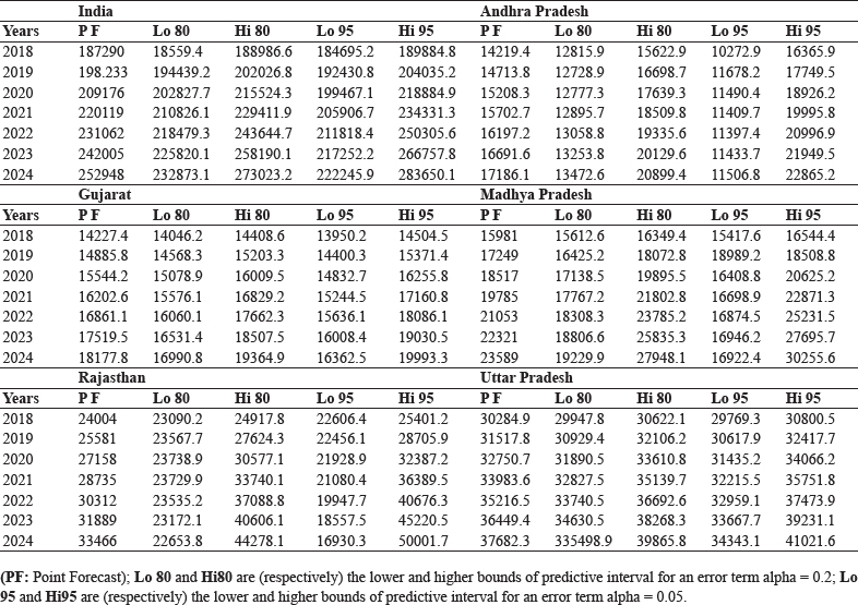
The forecasts details for milk production of these two time series are shown in Table (3) and Fig. (2). Statistically, an ARIMA(0,2,1) process is an equivalent to a Linear Exponential Smoothing (LES) model, Holt, (1957), Hyndman et al. (2008); with the Moving Average, MA(1) coefficient corresponding to the value 2 *(1 - a) in the LES model. We forecast that the milk production (respectively) in Gujarat and Uttar Pradesh may exceed the level of 18000 and 87000 in 2024/2025. The forecast intervals are less scattered in Uttar Pradesh compared to Gujarat, thus, the precision of prediction are best in Uttar Pradesh than Gujarat.
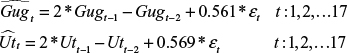
Table 3: Milk Production Forecasting: in Major states in India (In Miles tones)
Fig. 1 : Evolution of milk production in India Gujarat, Rajasthan, Andhra Pradesh, Madhya Pradesh and Uttar Pradesh over the period
Fig. 2 : Forecast results of Milk production in India Gujarat, Rajasthan, Andhra Pradesh, Madhya Pradesh and Uttar Pradesh over the period (2018-19-2024-25)
CONCLUSION
Diary sector is important activity of Agriculture sector. Milk production is having crucial role in development of dairy sector. Except the Uttar Pradesh, all major states and whole India register more than 2 percent growth rate during the study period. For all milk production data expect Andhra Pradesh, two time differencing required to make the data stationary in present investigation for forecasting purpose. From the forecasting figures, Uttar Pradesh followed by Rajasthan would play vital contribution in milk production in India. With 37.60 MMT in 2024-25 Uttar Pradesh would be leading state of India on milk production. To increase milk production need to provide quality fodder and proper health care of animals. This projection help to making strategy for future to meet our milk demand. For increasing the milk production need to make awareness to dairy owner and farmers on animal breeding program and healthcare practices.
REFERENCES
Anonymous. 2018. National Action plan of Diary development, Ministry of Agriculture & Farmers Welfare.
Anonymous. 2019. Department of Animal Husbandry, Dairying & Fisheries, Ministry of Agriculture and Farmers Welfare.
Bhardwaj, P.K., Pathera, A.K. and Bishnoi, S. 2017. Quality Evaluation of Milk Products Retailed in Hisar City of Haryana State. J. Anim. Res., 7 (3): 553-558.
Box, G.E.P. and Jenkins, G.M. 1976. Time Series Analysis: Forecasting and Control, Holden-Day. San Fransisco.
Chaudhari, D.J. and Tingre, A.S. 2015. Forecasting eggs production in India. Indian J. Anim. Res., 49(3): 367-372.
Deshmukh, S.S. and Paramasivam, R. 2016. Forecasting of milk production in India with ARIMA and VAR time series models. Asian J. Dairy Food Res., 35(1):17-22.
Engle, R.F. 1982. Autoregressive conditional heteroscedasticity with estimates of the variance of United Kingdom inflation, Econometrica., 50: 987-1008.
Gideon E.S. 1978. “Estimating the dimension of a model”. Ann. Statist., 6(2): 461-464.
Holt, C.C. 1957. Forecasting seasonal and trends by exponentially weighted moving averages. Office of Naval Research. Research Memorandum, pp. 52.
Hyndman, R.J. and Athanasopoulos, G. 2018. “Forecasting: principles and practice”, 2nd ed. OTexts, Melbourne, Australia. Section 3.4 “Evaluating forecast accuracy”. https:// otexts.org/fpp2/accuracy.html.
Hyndman, R.J. and Koehler, A.B. 2006. “Another look at measures of forecast accuracy”. Int. J. Forecasting, 22(4): 679-688.
Hyndman, R.J., Koehler, A.B., Ord, J.K. and Snyder, R.D. 2008. Forecasting with exponential smoothing: the state space approach. Berlin: Springer-Verlag.
Intriligator, M.D., Bodkin, R.G. and Hsio, C. 1996. "Econometric Models, Techniques, and Applications”. Prentice Hall edition.
Kwiatkowski, D., Phillips, P.C.B., Schmidt, P. and Shin, Y. 1992. “Testing the Null Hypothesis of Stationarity against the Alternative of a Unit Root”. J. Econometrics, 54 : 159-178.
Leybourne, S.J. and McCabe, B.P.M. 1994. A consistent test for a unit root. J. Busin. Econom. Statist., 12: 157-166.
Mishra, P., Fatih, C., Niranjan, H.K., Tiwari, S., Devi, M. and Dubey, A. 2020. Modelling and forecasting of milk production in Chhattisgarh and India. Ind. J. Anim. Res.,DOI- 10.18805/ijar.B-3918
Pablo, M.P. and Carlos, A.I. 2016. Forecasting with a Random Walk. J. Econom. Finan., 66 : 6.
Prajneshu. and Venugopalan, R. 1997. Statistical modelling for describing fish production in India. Indian J. Anim. Sci., 67 (5): 452-456.
Sharma, M., Jasrotia, N., Kumar, B., Bhat, A. and Mahajan, S., 2018. Modeling of Monthly Arrival of Rohu Fish using ARIMA in Jammu Region of J&K State. J. Anim. Res., 8(2): 259-262.